This page has the simple purpose of introducing you to the interest, loans and annuities based functions that Excel has built in to it that you might find of use in your work as an accountant.
The purpose of Excel’s in built functions is that they are fully comprehensive attempts at working out, for example, the interest implications you need to take into account in a variety of settings.
I am demonstrating these functions using Excel 2007: it will be different if you use an earlier version of the software.
Finding what Functions are Available
Open Excel and click on the Insert Function icon: it looks like this fx and is to be found on the left of the formula bar, as below.

This opens a dialogue box and to find out the categories of function available, click where it says or select a category … highlighted below. Choose from Financial functions, date and time, mathematics and trigonometry … and many more.
We are primarily interested in the financial functions and you are presented with the list of all of the financial function available in your version of Excel … there are many!

You should see the list beginning with ACCRINT, ACCRINTM ...
So rather than doing what I have just suggested, let’s target the functions we need specifically. That is, click on fx but this time enter depreciation in the Search for a function area then click Go and it provides you with a list of all in built functions that Excel thinks relate to that search string.
As you can see with the dialogue box here, it shows seven functions in Excel relating to interest although there are 31 in total:

You can also see here that when you highlight one of the functions, there is a short explanation of how that function works and what it does. So we can see that the ACCRINT function is the Returns the accrued interest for a security that pays interest at maturity. |
Please note: choose ACCRINTM, as a matter of interest and you will see that it is one of a group of functions that are not available by default. If this function is not available, and returns the #NAME? error, install and load the Analysis ToolPak add-in:
- Office Button
- Excel Options…
- Add-Ins on the left hand menu
Take a look at the graphic below to see what to do now to install the ToolPak by clicking the go button next to Manage Excel Add-Ins …

This now opens a dialogue box where you can now select the ToolPak Add-In:

Click OK now and note that you MIGHT have to insert your Office original CD into the drive to install this ToolPak. That #NAME? Error should have disappeared now: if not, close Excel and reopen it and it should have been solved!
Don’t forget, there is always a link to Excel’s Help files: it’s a hyperlink in blue at the bottom left of the dialogue box. Click on the link and it will explain in detail, with a fully worked example, what to do. The help file for ACCRINTM is:


You can even copy and paste the example into a worksheet and see the function in action.
Interest, Loans and Annuities
You are now aware of the choice of methods for dealing with interest, loans and annuities available as in built functions in Excel. What follows now is a brief review of some of them and some tips on how to set up a worksheet with any or all of the functions built into it.
The functions:
- FV = future value
- PV = present value
- PMT = payment
- PPMT = principal payment
- IPMT = interest payment
- ISPMT = payment interest
- RATE = interest rate per period
- NPER = number of periods
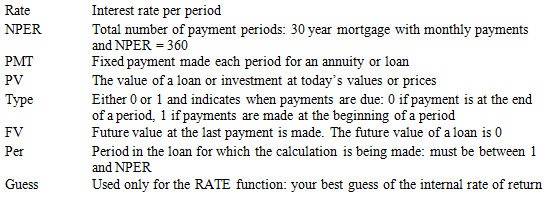
Of course, the chances are that you will not need to use all of these at any one time. I am demonstrating them at one time for convenience! The data we need to calculate and demonstrate these methods are:

Range Names
Before we take this any further, I want to introduce, or remind you of, range names because I am about to set up a worksheet that will allow you to calculate the provisions for depreciation using one or all of the above methods. However, I am assuming that the calculations will relate to the same asset at the same time etc therefore we will be providing for the same asset using the same basic data.
All we do to assign a range name is the highlight a cell or a range of cells that we would like to give a name to
Then whenever we need to call on or use that value or range, we just enter the range name in the formula or function we are using.
Like this:
I have assigned the range names … NB these relate to depreciation and you should change them if you wish to work with range names for the interest calculations
- cost to cell B11
- salvage to cell C11
- life to cell D11
Then for the SYD calculation, we would have:
=SYD(cost,salvage,life)
Now you don’t need to look for where the data are to be found, whatever you do to your worksheet and if you change the basic data, the formula automatically finds and updates itself and its result. More than that it doesn’t matter where in your worksheet or file you place your function either, using range names makes it really easy, just use those range names and Excel finds what you want.
Finally for now, if you open up the list of range names and click on any one of those names, the cursor goes to that range: again useful features if you have forgotten the name and where to find it.
Assigning Range Names
How do you set or assign range names? To assign a range name, highlight the cell or range you want to name and then type your chosen name in the name box:

If you close your spreadsheet and want to work on it again later but have forgotten which range names you have used in it, just click on the down arrow at the right of the name box and the list of names opens for you to use again. Excel never forgets these things!
If you redesign your worksheet or file, you can change the address of the range name … we’ll do that another time. If you are impatient, Excel’s Help files can sort this out with you.
The Interest, Loan and Annuity Spreadsheet
I have set up a really simple spreadsheet to cope with our chosen four methods: it looks like the following in which the range names are

Please note that some of the variables need to be entered as negative values. PMT, for example, the monthly payment amount is negative which reflects that fact that it is a cash outflow. Similarly with PV: as with capital budgeting, we assume here that the initial investment is a cash outflow and hence negative.
In this case, I have set up the spreadsheet for you and worked through all of the calculations: FV is £167,156.1 … what does that mean? PV is £3,790.79 … what does that mean? And PMT, PPMT and so on … what do they all mean?
I hope you have found this page useful and feel free to add your comments to this page to let me know the good and the bad!
Duncan Williamson