Introduction
This post is a comprehensive introduction to using Power Query Connections in Excel, especially using them to create Pivot Tables and Charts. There is no Excel file or video here but if you really need to learn how to do these things, this is one of the best explanations you will find.
As I have been working on some Power Query models, I have been thinking about aspects of them and Pivot Tables that I have not considered before. I also faced problems such as the percentages disappearing from a Query and the [Data.Format.Error] I faced when updating and refreshing a Query. I have created blog entries on both of those issues, by the way.
What is a Connection Only Query?
When we create a Query, we can click Close and Load to… and choose from the following list:
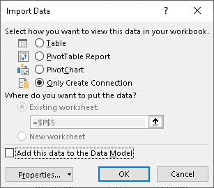
Choosing Only Create Connection will save the Query but it will be hidden: there will be no entry in any worksheet. That saves size and speed. When would you hide a Query? I do so when I create an intermediate table that I don’t need to see. For example, I have the raw data in a visible and I create a Query that I know I am going to use to create another table or to merge with another table. Things like that drive me to hiding an intermediate Query.
Once the Query is saved only as a connection, I asked the question: can I use it directly to create a Pivot Table or a Pivot Chart? The answer is yes you can use it to create those things and this is how!
Creating a Pivot Table from a Connection Only Query?
There are two ways to create a Pivot Table from a Connection Only Query:
- Using an Existing Connection
- Converting Connection Only to Normal Connection
Using an Existing Connection
Whether it’s for security reasons or to maintain a low file size, we can keep our connection only data hidden from view and create a Pivot Table from it. To do that, do this:
Insert Pivot Table

Click the radio button that says Use an external data source and then Choose Connection, after which you will see this dialogue box:
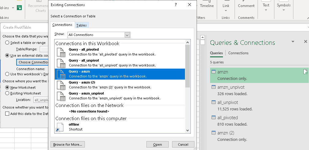
Providing you have created the connection that I am talking about, you should see it in the Connection in this Workbook list. Just click on the appropriate entry and then close and you will return to the Pivot Table dialogue box.
In the Pivot Table dialogue box, make sure you select create New Workbook or set the target cell for the start of the Pivot Table in the Existing Worksheet.
Click OK and you will see your Pivot Table ready and waiting for you.
Second Instance of your Query is Created
Please note, with the above approach, you will see that a second instance of the amzn query, in this case, is created but you can delete the first of those Queries as the Pivot Table is only working from the second one.
Pivot Chart from Connection Only
By the way, we can create a Pivot Chart from our Connection Only Query, too, in the same way as we have just done for the Pivot Table. Look at the following screenshots to see the slight differences between the two approaches:
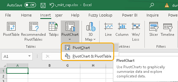
Firstly, though, when we start this process, on the Insert tab, it asks us if we want just a Pivot Chart or a Pivot Chart and Pivot Table: I have to confess, I don’t see the difference between them once they have been prepared. When we select Pivot Chart, we get a Pivot Chart and a Pivot Table. When we select Pivot Chart & Pivot Table, we get a Pivot Chart and a Pivot Table!
Here is the process:


Converting Connection Only to Normal Connection
Saving a Query to Connection Only does not, so to speak, condemn it to death or permanent dormancy because we can put it into the worksheet like this.
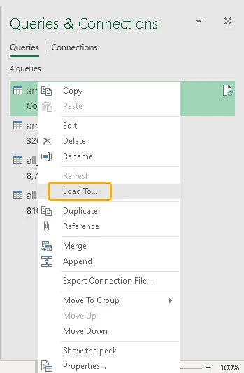
Right click on the connection only query in the Queries & Connections panel in the appropriate Excel file and click on Load to…
That will open up the dialogue box we have already seen but with a small difference:
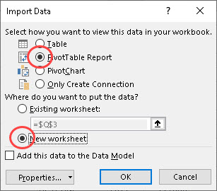
And rather than leaving Only Create Connection selected, change that to having PivotTable Report selected: just click on the radio button next to it, then click OK. That opens the following dialogue box, that is also probably already familiar to you:
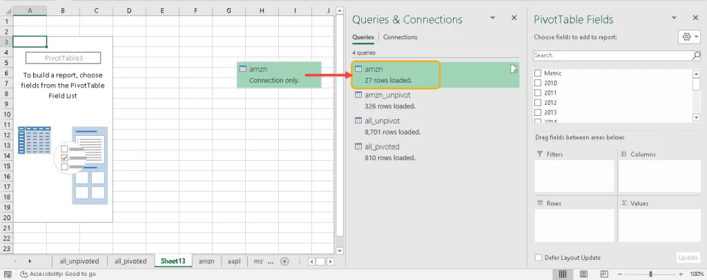
I have highlighted on that screenshot where it says 27 rows loaded, whereas previously it said connection only … look out for that.
Now you can prepare your Pivot Table and a Pivot Chart as you wish. If you just want a Pivot Chart and not a Pivot table, try this:
Right click the connection only link in the Queries & Connections pane and choose Pivot Chart rather than Pivot Table:
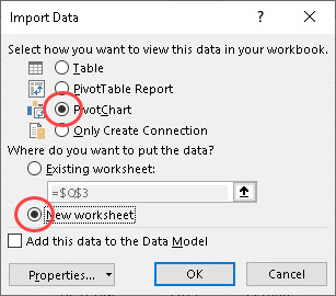
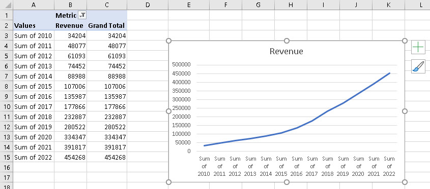
Providing your default chart can be drawn by a Pivot table, when I click OK, I am taken straight to the Pivot Chart worksheet that Excel has created for me:
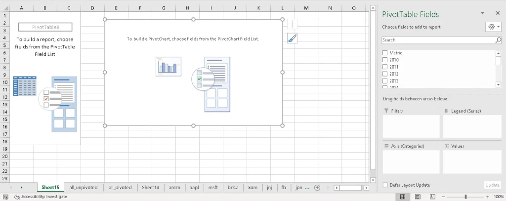
I can now populate my chart as I wish. Do notice that choosing the Pivot Chart does bring the Pivot Table with it!
What if my Default Chart is Incompatible with a Pivot Table?
I knew that, for example, Scatter (XY) charts cannot be created by Pivot Tables but I had forgotten that my default chart was a Scatter (XY) chart. So, when I tried to create a Pivot Chart from the instructions above, I was given this message:
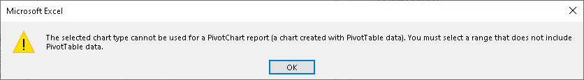
It created the Pivot Table as it gave me that message and I was easily able to create a Line chart for myself. However, I needed to change my default chart so that when I repeat this exercise, I can create the chart I want, immediately. See the next section for instructions on how to do that.
Changing your Default Chart in Excel
Create an example of the type of chart you would like to save as the Default chart and do the following, that starts with a Scatter (XY) chart:
- Click on the Insert tab
- Go to the bottom right hand corner of the Charts section and click on the button there
- That opens the dialogue box you see above
- Choose the type of chart you want to create as default, if it is not the one you want as Default
- Right Click on the version of the chart from the top row and it should show an icon saying “Set as Default Chart” … click on that and it should now be your Default chart.
To check that you have done this properly, click on some data, not necessarily in a Pivot Table and click Alt+F1 and your Default chart should appear.
Can I Hide my Query Again Once I Have Created my Pivot Table?
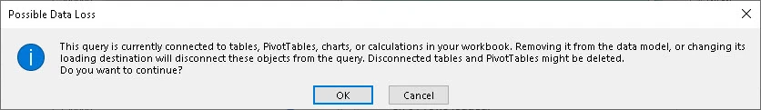
Finally, let’s assume we hid our Query for a reason: can we hide it again after we have finished with our Pivot Table/Chart? The answer is yes but if you do that, it will automatically delete the Pivot Table as it hides the Query again.
To do this, right click on the Query in the Queries & Connections panel, click Load to… and ask it to only create connection. It will tell you this:
That’s it. What happens when we work with a Connection, unhide it, hide it, create PivotTables and Charts and so on!
Duncan Williamson
7th March 2020
No comments:
Post a Comment